The fluxes between the Earth's surface and the atmosphere are usually called surface fluxes. Many processes are involved such as evaporation from land and sea, warming and cooling of the earth, emission and deposition of gases and particles.
Surface fluxes
The fluxes between the Earth's surface and the atmosphere are usually called surface fluxes. Many processes are involved such as evaporation from land and sea, warming and cooling of the earth, emission and deposition of gases and particles. These processes are vital to life and are being investigated in various scientific fields such as agriculture, bioclimatology, hydrology and meteorology.
Surface fluxes traditionally are measured by instruments mounted on meteorological masts. Typical measurement data are wind speed, air temperature, air humidity and concentration of gases (eg CO2) and particles at several levels above ground. Calculation of surface fluxes are done by classical similarity-scaling equations on turbulent flow in the atmospheric boundary layer. This method applies only for large homogeneous landscapes (of the order of kilometers).
Most landscapes are heterogeneous, ie consist of two or more land cover types in patterns. The patterns are partly a result of mankind activities: agriculture, urban growth and industrial elements, partly a result of geomorphological and climatic forcings: mountains, glaciers, deserts, lakes, rivers, soil types and vegetation systems.
Microscale flux aggregation model
The microscale flux aggregation model is based on a physical description of turbulent flow (Jensen 1994, Hasager 1997). The flow equations are linearized and only the diffusion term is modelled. A Fast Fourier Transform is used to solve the equations. The microscale model predicts area-integrated (effective) roughness values representative for mesoscale grid cells. It also predicts local values of friction velocity and land surface momentum flux in every pixel in a region. The model constitutes an alternative to the so-called heuristic blending height method (Mason 1988).
To calculate the friction velocity pixelwise the following inputs are nessecary:
the landscape roughness defined as z0(x,y)
the wind speed and wind direction at the computational level U(z)
|
Roughness map z0(x,y)
|
Momentum flux map u*²(x,y)

|
This schematic illustrates the microscale model step very simply. As the Fourier solution method assumes the landscape pattern to be repeated infinetely, this is symbolized with the open-ended landscape boxes.
Surface heat flux heat will in the future be calculated in a similar way. The nessecary inputs for heat flux calculations are in addition to the roughness maps, maps of surface temperatures. These are available from satellite sensors measuring the thermal infrared radiation.
The future version of the microscale flux model aims at the prediction of heat, water vapour and passive scalar fluxes. Prediction of land surface deposition of pollutants will be possible by inverting the model. Such downscaling require grid mean concentrations of the pollutant as input.
A demonstration case from the Rhine Valley, Germany
In the so-called TRACT project (Transport of Pollutants over Complex Terrain) a 100 km * 100 km area in South-west Germany including parts of France and Switzerland was monitored from field sites, airborne instruments and satellites. The project was funded within the 4th framework programme of the EU commission.
Part of the project focused on surface flux retrieval in highly heterogeneous landscapes. The model was developed within this subproject. In real terrain the boundary condition of roughness is a major topic. The reason is that it is not practically possible to map an extended area from field surveys. Traditional topographic maps do not hold spatial information at a relevant level. Therefore the line of action is to analyse spatial data from satellite sensors.
In the present project multi-temporal classification of Landsat TM scenes (Konrad et al. 1994) was carried out. The high-resolution images gave a reliable source of information of the land cover. At the same time traditional micrometeorological data of the aerodynamic roughness was measured in most of the land cover classes present within the study area (Fielder et al. 1994)..
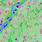
Classification results from Landsat TM is shown for a 15 km * 15 km area in the Upper Rhine Valley in 1993. The result was 19 cover types and one "reject" which is clouds.
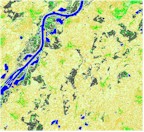
As the aerodynamic roughness is known in every land cover class, it is simple to assign these values and obtain a roughness map. The surface roughness map from 1993 of the Upper Rhine Valley, Germany is shown below.
The roughness map is used as input to the microscale aggregation model and the output is friction velocity perturbations pixelwise. From these we calculate the land surface momentum flux maps. These high-resolution momentum flux maps may be the first of their kind.
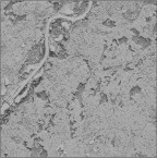
Land surface momentum flux in the Rhine Valley, Germany as calculated by the microscale aggregation model. The case is for a wind speed of 4 m s-1 at 4 m height above ground from the North.
The map show a large momentum flux above forests. At the leading edges the maximum response is found. This is in accordance with theoretical knowledge and field data. When the air moves from a smooth surface to a rougher surface, a very large increase in the momentum flux occurs. At contrary a very low momentum flux occurs when the air moves from a rough surface to a smoother.
A display of the friction velocity response along a selected horizontal line from the North to the South in the direction of the wind, is given. A black line shows the position in the momentum flux map.
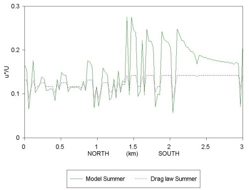
The profile shows the microscale model results of the friction velocity and the hypothezed equilibrium values calculated by the geostrophic drag laws. Equilibrium conditions can only be expected in landscapes with very large homogeneous patches of the order of 10-20 km. The first 1.5 km of the landscape is mixed agriculture with small patches of vine, corn, meadow among others. In this terrain the momentum flux is moderately fluctuating. At 1.5 km downstream the wind meets forest Strüt. This large forest has a very large momentum flux at the leading edge, then a gradual decline downstream.
References
1. Fiedler, F. Ebert, J. Noppel, H. and Adrian, G. 1994 Heat exchange processes at sloping terrain, Annual report 1994, Universitat Karlsruhe, 42-73.
2. Hasager, C.B. 1997 Surface fluxes in heterogeneous landscape. Risø-R-922 (EN). ISBN 87-550-22118-9, ISSN 0106-2840, ISSN 0906-1797.
3. Hasager, C.B. & Jensen, N.O. 1999 Surface-flux aggregation in heterogeneous terrain, Q.J.R. Meteorol. Soc. 125, 2075-2102.
4. Jensen, N.O. 1994 Flux-aggregation modelling. European Geophysical Society XIX General Assembly (Session OA18), Grenoble, France, April 1994.
5. Jensen, N.O.; Hasager, C.B.; Hummelshøj, P.; Pilegaard, K.; Barthelmie, R.J., Surface flux variability in relation to the mesoscale. In: Exchange and transport of air pollutants over complex terrain and the sea. Larsen, S.E.; Fiedler, F.; Borrell, P. (eds.), (Springer-Verlag, Berlin, 2000) (Transport and chemical transformation of pollutants in the troposphere, v. 9) p. 322-328
6. Konrad, C. Segl, K. and Wiesel, J. 1994 Multitemporal land-use classification of the Upper Rhine Valley and adjacent areas with Landsat TM image data. In F.Fiedler Final report, Institut für Meteorologie, University of Karlsruhe a1-a13.
7. Mason, P.J. 1988 The formation of areally-averaged roughness lengths, Q.J.R.Met.Soc. 114, 399-420.
Funding
- European Union 4. programme
- The Danish Environmental Research Programme
- The Danish Research Academy
Completed