|
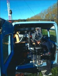
The Risø mini lidar system consists of
- A pulsed laser system (water cooled)
- A Cassegrain telescope with filters and detectors
- A digital sampling/storage scope
- A stepper motors w/ controllers for scanning (azimuth and declination)
- A PC control and data acquisition and storage system
- A mini Van (Ford Transit)
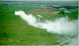
The ground based Risø Mini lidar system is used to quantify aerosol concentrations in the atmosphere. It is sensitive enough to detect natural occurring aerosol backscatter from single laser shots in the range 50 - 500 meters. During controlled diffusion tests, however, it measures backscatter from artificially generated smoke puffs and plumes, which we turn into calibrated aerosol concentrations, see below.
|
 |
The lidar principle of operation is much like conventional radar except that it uses a pulsed infrared laser beam instead of radio waves. A short light pulse is emitted by the laser and the echo is recorded by the storage scope. The position is given by the time delay of the echo and the strength of the echo is related to (see below) the aerosol particle concentration at that position. From a single laser pulse, typically 500 simultaneous sampling points (range gates) are recorded along the beam path. The detector and the laser beam are built coaxial in the telescope. The telescope (with laser head and detector) can be turned along two axes (azimuth and declination) by means of stepper motors.
The lidar head with telescope, detector and laser head can scan vertically between two pre-set turn angles in order to scan cross-sections of continuous smoke plumes. Each vertical scan consists typically of 20 laser shots covering angles between 0° and 20° (sometimes smaller angles are used). A scan typically lasts 1 sec with 20 or 40 rays covered per scan. The turn around time is approximately 1.5 seconds between the scans. The pause is used to decelerate and accelerate the telescope and to transfer data to the PC.
During continuous smoke plume experiments, the radial distance between range gates was 0.75 m (sampling rate 200 Ms/s). This corresponds to a Nyquist sampling length of 1,5 meters consistent with the detector systems overall spatial bandwidth (see technical specifications).
Range gates separation as small as 37.5 cm (400 Ms/s) can be achieved, and smoke plumes can be scanned at distances from ~100 meters in front of the lidar head up to distances several kilometres away. Typically, experiments with artificial smoke plumes were scanned or measured at distances ranging from 200 to 800 meters from the laser head.
From Lidar returns to aerosol concentrations
Lidar's principle of operation
A short light pulse with high energy (effectively ~1.5 meters long with ~10 mJoule energy is emitted from the laser head and fed into the lidar systems coax centreline.
The backscatter from aerosols in the beam path is then detected and digitised by the scope. The distance from the lidar head to the aerosols r is then given by the time delay of the echo to for each range gate, and the strength of the echo at range r, the received power P(r), is related to the aerosols effective volumetric backscatter coefficient b through the lidar equation.
The lidar equation
The interpretation of lidar returns in terms of aerosol concentrations are based on the theory of propagation of electro-magnetic radiation and attenuation in an optically dense media.. The lidar equation accounts for this process:
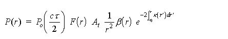
P(r) is the power received from the range r = ct/2, where c is the speed of light. The "½" factor arises from pulse travelling to the distance r and back to the receiver in time t. Po is the power transmitted at time zero. The effective length of the laser pulse is ct/2, where t is the lasers pulse duration. At is the effective area of the telescope, and divided by r2 this term defines the solid angle acceptance. The design with the laser pulse emitted in front of the telescope (coaxial) results in a simple geometric transmitter/receiver overlap function, F(r), which accounts for the effective overlap of the receivers field of view with the laser pulse. (This factor is only of importance at the shortest ranges, r <100).
b(r) [Sr-1 m-1] denotes the volumetric (per unit volume) backscatter coefficient of the atmosphere at range r, and k(r) [m-1] is the corresponding extinction coefficient.
The volumetric backscatter coefficient defined the fraction of incident energy scattered per solid angle in the backward direction (180°), per unit length. The volume extinction coefficient k defines correspondingly the fraction of the energy flux that is lost per unit length during the propagation.
In general, both the backscatter and the extinction properties depend on wavelength, particle size, and the optical properties of the aerosols.
The lidar equation (1) applies to relatively transparent medium where an only single scattered light is accounted for.
The lidar equation therefore relates the backscatter and extinction coefficients range dependence to the lidar return signal P(r), and the optical geometry of the transmitter and receiver units.
Data processing
Backscatter to Extinction ratio, and Concentration
Given a measured lidar return profile P(r), the lidar equation (1) becomes a first order integral equation with two unknown quantities, b(r) and k(r).
In order to solve this equation, a linear relationship between b(r) and k(r) is next introduced, based on Mie scattering theory as applied to elastic scattering on spherical particles (Bohren, 1983). This closed the lidar equation.
For single-scatter processes, the backscattered intensity is furthermore proportional to the number of particles per unit volume, that is, to the particle density. Puffs or smoke plumes internal aerosol concentrations can therefore, to first order, be interpreted as being proportional to the lidar systems inferred backscatter coefficient b(r), provided that the optical properties of the aerosols (e.g. the smoke particles size distribution) will not change during measurement trials (½-1 hr).
During stationary meteorological conditions with respect to background aerosol level and humidity, we assume that the particles size distribution is constant, and consequently proportionality between backscatter and aerosol concentration is obtained.
|
Artificial smoke generation
Artificially generated aerosol plumes (smoke) was used during all the experiments.
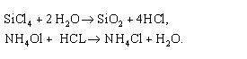
A smoke generator produced a continuous release of sub-micron aerosol particles consisting of a conglomerate of SiO2 and NH4Cl, which could easily be detected by the lidar system.
Mixing SiCl4 and a 25% solution of NH4OH in their neutralising, stoiciometric ratio (1:3.2) in a strong air stream (jet), the two liquids reacts instantaneous as follows:
|
|
Stable and strong artificially smokes plumes were in this way generated for the experiments. In situ Measurements on the artificial smoke particles size distributions, taken from both the plume's centre-line and from its sides, turned out to be remarkably constant both with time and with respect to its shape.
REFERENCES
- Jørgensen, H.E.; Mikkelsen, T.; Streicher, J.; Herrmann, H.; Werner, C.; Lyck, E., Lidar calibration experiments. Appl. Phys. B (1997) 64, 355-361
- Jørgensen, H.E.; Mikkelsen, T., Lidar measurements of plume statistics. Boundary-Layer Meteorol. (1993) 62, 361-378
- Cionco, R.M.; aufm Kampe, W.; Biltoft, C.; Byers, J.H.; Collins, C.G.; Higgs, T.J.; Hin, A.R.T.; Johansson, P.E.; Jones, C.D.; Jørgensen, H.E.; Kimber, J.F.; Mikkelsen, T.; Nyren, K.; Ride, D.J.; Robson, R.; Santabarbara, J.M.; Streicher, J.; Thykier-Nielsen, S.; Raden H. van; Weber, H., An overview of MADONA: A multinational field study of high-resolution meteorology and diffusion over complex terrain. Bull. Am. Meteorol. Soc. (1999) 80, 5-19
For further information, please contact Torben Mikkelsen